|
Home
Introduction
Screen Shots
Download
Order
|
|
There
are over 100 examples included in the package. The follows will
show you only a few of them. You may see how fast and how easy for
Auto2Fit to solve theose problems.
1:
Regression and Curve Fit
Unlike
most of other regression/curve fit softwares, the computation
engine of Auto2Fit is based on Evolution Algorithms rather than
Least Square or Levenberg-Marquardt Algorithms. This makes Auto2Fit
very robust and flexible to meet all type of regression problems
with any complicated functions. All the Statistical Reference Datasets Project (SRDP) of the National Institute of
Standards and Technology (NIST)
can be solved effortless, even without using suggested
initial start values. The examples belows are some
ones very hard or impossible to be fitted by other regression
softwares (in the cases that the start values are unknown), but so easy for Auto2Fit.
1.1:
MountCurve - Nonlinear Regression Problem
The
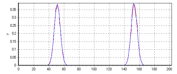
curve function required to be fitted is defined as:

The
data can be viewed here. There are two variables:
x and y, and three parameters: m1, m2 and m3. The function is
not so complicated, but it is not easy to find proper values
of parameters by conventional methods. You may try other nonlinear
regression softwares or tools.
Within
1000 iterations, you will get prefect answer
| Codes
in Auto2Fit
|
Results
from Auto2Fit
|
| Title
"Mounttain Curve Fit";
Variables
x, y;
Parameters
m1, m2, m3;
Function
y = m1 / m2 * exp(-0.5 * sqr((x - m3) / m2));
Data;
400 0.00000
401 0.00000
402 0.00000
403 0.00000
.
.
499 0.00000
500 0.00000
501 0.00000
|
"Mounttain
Curve Fit"
Iterations:
857
Elapsed
Time (Hr:Min:Sec:Msec): 00:00:04:170
Algorithms:
Maximum Inherit Optimization (Scheme 3)
Stop
Reason: stoped by user
Root
of Mean Square Error (RMSE): 0.005028842682
Sum
of Square Error (SSE): 0.005159008779
Correlation
Coef. (R): 0.9985732835
Determination
Coef. (DC): 0.9971484642
m1:
1.541309057
m2:
4.017358503
m3:
450.8919547
======
Output Results =====
|

Return
to top
1.2:
Cos Function - Multi-nonlinear Regression Problem
The
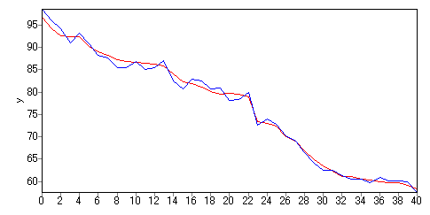
curve fit function is defined as:

There
are four variables: x1, x2, x3 and y, and three parameters:
m1, m2 and m3. The data can be viewed here.
| Codes
in Auto2Fit
|
Results
from Auto2Fit
|
| Title
"CosSin - Regression";
Variable
x1, x2, x3;
Variable
Y;
Parameter
m1, m2[0, 1000], m3;
Function
y = ((m1 / x1) - cos(m2 * x2)) * x3 * m3 / x1;
Data;
0.5797 2.5708 5.0022 98.5408
0.5797 2.4431 4.8947 95.8701
0.5797 2.5916 5.0202 94.2456
0.5797 2.5611 4.9939 91.0629
.
.
0.5797 1.9958 4.5539 60.0994
0.5797 2.3907 4.852 59.9757
0.5797 1.8992 4.4871 57.5347
|
"CosSin
- Regression"
Iterations:
5001
Elapsed
Time (Hr:Min:Sec:Msec): 00:00:04:780
Algorithms:
Differential Evoluation(Scheme 1)
Stop
Reason: auto-detected
Root
of Mean Square Error (RMSE): 1.011115788
Sum
of Square Error (SSE): 41.91656063
Correlation
Coef. (R): 0.9965554089
Determination
Coef. (DC): 0.9930915321
m1:
2.492258238
m2:
49.99801377
m3:
2.132265565
======
Output Results =====
|

Return
to top
1.3:
SinCos Function - Multi-nonlinear Regression Problem
Function
defination:

There
are total 4 variables: one denpendent variable y and three
independent variables x1, x2 and x3, four parameters: a1, a2,
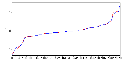
a3 and a4. The data can be viewed here.
This
regression problem is a little hard for other algorithms, for
example, Gauss-Newton or Levenberg-Marquardt
methods, but rather easy for Auto2Fit.
| Codes
in Auto2Fit
|
Results
from Auto2Fit
|
|
Title
"SinCos Function9 - Multi Nonlinear Regression";
Variables
x1, x2, x3, y;
Parameters
a1, a2, a3, a4;
Function
y=(a1+x1/a2+cos(a3*x2/x3))/(a4*sin(x1+x2+x3));
Data;
0.2671 8.1681 0.4279 -0.0800
0.0166 1.3885 1.6640 -1.1242
0.6063 6.8171 1.7050 0.8925
.
.
0.3932 2.6776 2.4910 -0.3780
0.5714 8.2727 1.2285 -0.2521
0.4258 0.8845 2.0383 -0.6213
|
"SinCos
Function - Multi Nonlinear Regression"
Iterations:
370
Elapsed
Time (Hr:Min:Sec:Msec): 00:00:00:830
Algorithms:
Maximum Inherit Optimization (Scheme 3)
Stop
Reason: stoped by user
Root
of Mean Square Error (RMSE): 0.02516162826
Sum
of Square Error (SSE): 0.03861955973
Correlation
Coef. (R): 0.998701447
Determination
Coef. (DC): 0.9974045694
a1:
0.4933689555
a2:
2.937520807
a3:
10.99995909
a4:
5.837467985
======
Output Results =====
|

Return
to top
1.4:
Regression Demo 12 - Multi-nonlinear Regression of Implicit
Function
The
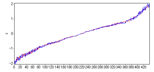
implicit function
is defined as:

There
are total 3 variables: one dependent variable z and two
independent variables x, y, three parameters: a, b amd c. The data file
is included in the package.
The
particular points for this problem is the function is in implicit
type.
| Codes
in Auto2Fit
|
Results
from Auto2Fit
|
|
Title
"Regression Demo 12 - Nonlinear Regression
for Implicit Function";
Variable
x, y, z;
Parameter
a, b, c;
Function
z = sin(z-a*x)*cos(z-b*y)-cos(c*x+y);
Data;
//x y z
-0.7 1.4 -1.9033
-0.85 1.4 -1.8437
.
.
0.2 2.8 1.7662
1.25 0.6 1.8032
|
"Regression
Demo 12 - Nonlinear Regression for Implicit Function"
Iterations:
752
Elapsed
Time (Hr:Min:Sec:Msec): 00:00:10:880
Algorithms:
Differential Evoluation(Scheme 1)
Stop
Reason: stoped by user
Root
of Mean Square Error (RMSE): 0.0814499163
Sum
of Square Error (SSE): 2.918999101
Correlation
Coef. (R): 0.9961258054
Determination
Coef. (DC): 0.9922647652
a:
0.5032554508
b:
3.007669859
c:
2.009839861
======
Output Results =====
|

Return
to top
1.5:
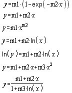
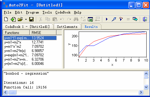
Curve Fit
There
are 7 functions needed to be fit, with parameter number form
2 to 3. Of course, you may add any more functions you want to
fit with any complication, just remember to declare the
parameters you will use.

| Codes
in Auto2Fit
|
Results
from Auto2Fit
|
|
//Non-linear
regression
Title
"BoxBod - Regression";
Variable
X, Y;
Parameter
m1, m2, m3;
Function
y=m1*(1-exp(-m2*x));
Function
y=m1+m2*x;
Function
y=m1*x^m2;
Function
y=m1+m2*ln(x);
Function
ln(y)=m1+m2*ln(x);
Function
y=m1+m2*x+m3*x^2;
Function
y=(m1+m2*x)/(1+m3*ln(x));
//add
more functions with any type which you want to fit
Data;
1 109
2 149
3 149
5 191
7 213
10 224
|

|
Return
to top
1.6:
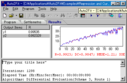
Nonlinear Regression for Multi-Outputs
One
of special features of Auto2Fit is it capable of doing regression
for the problems with more than one dependent
variable. In the following example, there are three independents:
X1, X2 and X3, two dependents: Y1 and Y2, and four parameters
a, b, c and d. The data can be viewed here

| Codes
in Auto2Fit
|
Results
from Auto2Fit
|
|
Title
"Type your title here";
Parameters
a, b, c, d;
Variable
x1, x2, x3, y1[output], y2[output];
StartProgram;
var
i:integer;
begin
for
i:=0 to datalength-1 do begin
y1[i]:=x1[i]^a+b*LN(x2[i])*EXP(x3[i]^c);
y2[i]:=x1[i]*a+b*exp(x2[i]^d)*ln(x3[i]^c);
end;
end;
EndProgram;
Data;//x1,
x2, x3, y1, y2
1 0.9874667 0.98746 0.915695 0.2367
2 0.6184713 1.23694 -2.90142 0.7088
.
99 98.47721 9749.244 172.9479 38.723
100 79.5060 7950.601 159.8588 35.861
|

|
Return
to top
2:
Function Optimizations
Both
unconstrained and constrained function optimization problems
can be solved by Auto2Fit in a simple way
2.1:
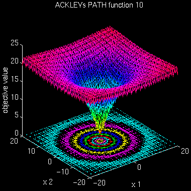
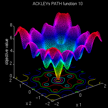
Ackley's Path function - Global Optimization Problem
Ackley's
Path is a widely used multimodal test function. The function
is defined as:

where
a = 20; b = 0.2; c = 2*pi; i =1:n; -32.768 <= x(i) <=
32.768.
The
global minimum is: f(x) = 0; x(i) = 0, i = 1:n.
Codes in Auto2Fit
|
Title
"Ackley's Path function";
Constant
a = 20, b = 0.2, c = 2*pi, n = 20;
Parameters
x(1:n) [-32.768, 32.768];
Minimum
= true;
Function -a
* exp(-b * sqrt(1/n * sum(i = 1:n) (x[i]^2))) -
exp(1/n * sum(i = 1:n) (cos(c * (x[i])))) + a +
exp(1);
|
That's
all. Run it, within 1 seconds, the results will looks like:
|
"Ackley's
Path function"
======
Results ======
Iterations:
1001
Elapsed
Time (Hr:Min:Sec:Msec): 00:00:00:500
Stop
Reason: Maximum iterations reached
Algorithms:
Maximum Inherit Optimization (Scheme 3)
x1:
-1.56365587213379E-15
x2:
-5.01293370084778E-16
x3:
-3.19937359425478E-16
x4:
2.69211471782096E-15
x5:
-2.78823957190795E-16
x6:
4.19667976836696E-15
x7:
2.74358251530853E-15
|
x8:
1.09470827859725E-15
x9:
-1.02306165823084E-15
x10:
-1.61013988033348E-15
x11:
1.62620916215995E-15
x12:
-5.80951025602165E-16
x13:
-1.26472212025188E-16
x14:
5.92338829520887E-16
x15:
-1.53196863198793E-15
x16:
-5.09898751730622E-15
x17:
-4.83550571903038E-15
x18:
-1.3068975607019E-15
x19:
1.73505732732911E-15
x20:
-3.46806402565796E-15
Min.
Value: 7.54951656745106E-15
======
Finished ======
|
Return
to top
2.2:
Alex Function 1 - Global Optimization Problem
The Alex function 1 is an optimization problem to
find global minimum value. The function is defined as

Where -100 <= x(i) <= 100
there are four local minimum at:
-
f(x1,x2) = -1; (x1, x2) = (pi, pi);
-
f(x1,x2) = -1.1; (x1, x2) = (2*pi, 2*pi)
-
f(x1,x2) = -1.2; (x1, x2) = (3*pi, 3*pi)
-
f(x1,x2) = -1.3966; (x1, x2) = (12.9977, 12.9977)
one global minimum at
-
f(x1,x2) = -1.5047; (x1, x2) = (11.9664, 11.9664).
Since the global minimum has a small area relative to the local minimum space
and search space. It is quite easy to trap into local best
Codes
in Auto2Fit
|
Title
"Alex function 1";
Constant
M = 100;
parameter
x1[-M, M], x2[-M, M];
Minimum=true;
function
-cos(x1) * cos(x2) * exp(-((x1 - pi)^2 + (x2 - pi)^2))
-1.1
* cos(x1) * cos(x2) * exp(-((x1 - 2 * pi)^4 + (x2
- 2 * pi)^4))
-1.2
* cos(x1) * cos(x2) * exp(-((x1 - 3 * pi)^6 + (x2
- 3 * pi)^6))
-1.3
* cos(x1) * cos(x2) * exp(-((x1 - 3.5 * pi)^6 +
(x2 - 3.5 * pi)^6))
-1.4
* cos(x1 * pi) * cos(x2 * pi) * exp(-((x1 - 4 *
pi)^8 + (x2 - 4 * pi)^8));
|
Results
|
"Alex
function 1"
======
Results ======
Iterations:
1001
Elapsed
Time (Hr:Min:Sec:Msec): 00:00:00:330
Stop
Reason: Maximum iterations reached
Algorithms:
Genetic Algorithms
x1:
11.966377833722
x2:
11.966377833722
Min.
Value: -1.50470334517049
======
Finished ======
|
Return
to Top
2.3:
Alex Function 5 - Global Optimization Problem
Function
defination:

There
are three local best: f(x) = 0.095647 at (2.9425, 1.91849),
f(x) = -0.53083 at (-3.72329,-3.2188), f(x) = -0.75590 at (3.62126,-1.51937), and
one global best at f(x) = -0.96085 at (-2.78765 ,3.11559),
| Codes
in Auto2Fit
|
Results
from Auto2Fit
|
|
Title
"Alex Function 5 - Global OPtimization";
Parameters
x1[-150, 150], x2[-150, 150];
Minimum
= true;
Function
(x1^2+x2-11)^2+(x1+x2^2-7)^2+sin(x1^2+x2^2);
|
"Alex
Function 5 - Global OPtimization"
======
Results ======
Iterations:
160
Elapsed
Time (Hr:Min:Sec:Msec): 00:00:00:220
Stop
Reason: Auto-detected
Algorithms:
Maximum Inherit Optimization (Scheme 3)
x1:
-2.78765148360219
x2:
3.1155938532805
Min.
Value: -0.960854346462801
======
Finished ======
|
Return
to top
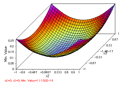
2.4:
Griewangk's
function
Function
defination:
| Codes
in Auto2Fit
|
Results
from Auto2Fit
|
|
Title
"Griewangk's function";
Const
n = 30;
parameter
x(1:n)[-600,600];
Minimum=true;
function
sum(i=1:n)(x[i]^2/4000)-prod(i=1:n)(cos(x[i]/sqrt(i+1)))+1;
|
"Griewangk's
function"
======
Results ======
Iterations:
1213
Elapsed
Time (Hr:Min:Sec:Msec): 00:00:02:30
Stop
Reason: Auto-detected
Algorithms:
Differential Evoluation(Scheme 1, Route 1)
x1:
5.19086848914639E-11
x2:
-1.5298049972672E-8
...
x29:
-3.44025650328254E-8
x30:
-2.46452573845116E-8
Min.
Value: 1.11022302462516E-16
|
Return
to top
2.5:
Constrained Function
Finding
minimum value of:

subject
to

| Codes
in Auto2Fit
|
Results
from Auto2Fit
|
|
Title
"G0 function - Constrained Optimization";
Parameters
x(1:9)[0,1], x(10:12)[0,10], x13[0,1];
Minimum=true;
Function
5*sum(i=1:4)(x[i]-x[i]^2)-sum(i=5:13)(x[i]);
2*x1+2*x2+x10+x11<=10;
2*x1+2*x3+x10+x12<=10;
|
"G0
function - Constrained Optimization"
======
Results ======
Iterations:
2505
Elapsed
Time (Hr:Min:Sec:Msec): 00:00:00:990
Stop
Reason: Auto-detected
Algorithms:
Differential Evoluation(Scheme 1, Route 1)
x1:
1.53808620232974E-17
x2:
2.05910171482306E-16
x3:
3.44483160794896E-17
x4:
4.33187907080207E-16
x5:
1
x6:
1
x7:
0.999999999999997
x8:
0.999999999999999
x9:
1
x10:
2.51904270007037E-16
x11:
10
x12:
10
x13:
1
Min.
Value: -26
Constrained
Functions
2*x1+2*x2+x10+x11-(10)
= -3.698476469
2*x1+2*x3+x10+x12-(10)
= 1.195812712
======
Finished ======
|
3:
Equation Solve
Auto2Fit
can solve any linear, nonlinear equation or system equations
with any dimension and any complication, even the unanalytical
equations that are failed to be solved by the default solver
of some famous math softwares, for example, Mathematical, Maple,
MuPad and Scilab
3.1:
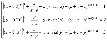
Nonlinear System Equation 1
Defination
of system equation:

| Codes
in Auto2Fit
|
Result
from Auto2Fit
|
|
Title
"Nonlinear System Equations";
Parameters
x, y, z;
Function
(x-0.3)^y^z+x/y/z-x*y*sin(z)+(x+y-z)^cos(x-1) =
1;
(y-0.2)^z^x+y/z/x-y*z*sin(x)+(y+z-x)^cos(y-2)
= 2;
(z-0.1)^x^y+z/x/y-z*x*sin(y)+(z+x-y)^cos(z-3)
= 3;
|
"Nonlinear
System Equations"
======
Results ======
Iterations:
194
Elapsed
Time (Hr:Min:Sec:Msec): 00:00:00:600
Stop
Reason: Auto-detected
Algorithms:
Differential Evoluation(Scheme 5, Route 1)
x:
1.46345419773711
y:
1.5967175598944
z:
1.84379181044959
Min.
Error: 8.88178419700125E-16
======
Finished ======
|
Return
to top
3.2:
Nonlinear System Equation 2
The
nonlinear system equations are defined as:

The
objective is to find roots of x, y and z
| Codes
in Auto2Fit
|
Result
from Auto2Fit
|
|
Title
"Three Dimension System Equations - Equation
Solve";
Parameter
x, y, z;
Function
x^2.23 + 2^sin(y) - 1.25 - z;
2
* x + y - 7 + 5.5 * z;
x
- y + 0.2 * z;
|
"Three
Dimension System Equations - Equation Solve"
======
Results ======
Iterations:
245
Elapsed
Time (Hr:Min:Sec:Msec): 00:00:00:280
Stop
Reason: Auto-detected
Algorithms:
Differential Evoluation(Scheme 5, Route 1)
x:
0.684082356686675
y:
0.857687722649482
z:
0.86802682981403
Min.
Error: 1.38777878078145E-16
======
Finished ======
|
Return
to top
3.3:
Nonlinear System Equation 3
This
system equations are little hard to be solved.

| Codes
in Auto2Fit
|
Result
from Auto2Fit
|
|
Title
"Equation Solve Demo 2 - Equation Solve";
Parameters
x1, x2;
function
(x1+2)^2-x2+sin(x1*x2)-6 = 0;
(x1^2+x2-11)^2+(x1+x2^2-7)^2-x1^x2-10
= 0;
|
"Equation
Solve Demo 2 - Equation Solve"
======
Results ======
Iterations:
490
Elapsed
Time (Hr:Min:Sec:Msec): 00:00:00:270
Stop
Reason: Auto-detected
Algorithms:
Differential Evoluation(Scheme 8, Route 1)
x1:
0.0636876933874153
x2:
-1.85933319070397
Min.
Error: 0
======
Finished ======
|
Return
to top
3.4:
Nonlinear Equation 4
This is a hydraulic equation
describing the relation between discharge Q and water depth
h, where m and b are constant

| Codes
in Auto2Fit
|
Result
from Auto2Fit
|
|
//Equation
solve
Title
"Hydraulic Function"; //Equation
solve for h
Const
b=5, m=1;
Const
Q=10; //discharge
Parameters
h; //water depth
Function
((b+m*h)*h)^3/(b+2*m*h)=Q^2/9.8;
|
"Hydraulic
Function"
======
Results ======
Iterations:
109
Elapsed
Time (Hr:Min:Sec:Msec): 00:00:00:160
Stop
Reason: Auto-detected
Algorithms:
Differential Evoluation(Scheme 8, Route 1)
h:
0.706184736292807
Min.
Error: 1.77635683940025E-15
======
Finished ======
|
Return
to top
3.5:
linear System Equation
The linear system equations are
defined as:

| Codes
in Auto2Fit
|
Result
from Auto2Fit
|
|
Title
"System Linear Equations";
Parameters
x1, x2, x3, x4;
Function
0.78*x1-0.02*x2-0.12*x3-0.14*x4=0.76;
-0.02*x1+0.86*x2-0.04*x3+0.06*x4=0.08;
-0.12*x1-0.04*x2+0.72*x3-0.08*x4=1.12;
-0.14*x1+0.06*x2-0.08*x3+0.74*x4=0.68;
|
"System
Linear Equations"
======
Results ======
Iterations:
243
Elapsed
Time (Hr:Min:Sec:Msec): 00:00:00:280
Stop
Reason: Auto-detected
Algorithms:
Differential Evoluation(Scheme 1, Route 1)
x1:
1.53496503496504
x2:
0.12200956937799
x3:
1.97515642252484
x4:
1.41295546558704
Min.
Error: 1.11022302462516E-16
Constrained
Functions
======
Finished ======
|
Return
to top
4:
Auto-Calibration
4.1:
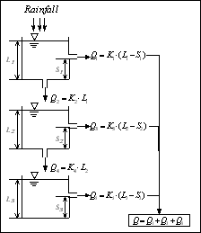
Tank Model
The
Tank Model is a conceptual rainfall-runoff model. Like illustrated in Figure
below, the Tank Model consists of several tanks arranged vertically in series
and each tank has one or more side outlets for runoff and a bottom outlet foe
vertical water movement to the next tank. The number of tank and side outlets
should be decided by consideration of actual watershed. In example here, there
are three tanks and each tank has only one side outlet.

The input to the model is rainfall, and the output is runoff.
The parameters used in the model are described as followings:
- Storage
capacity of each tank: S1, S2 and S3 (total 3)
- Initial
storage of each tank: L1, L2 and L3 (total 3)
- Discharge
coefficient: K1, K2, K3, K4 and K5 (total 5)
- Catchment
area: Area (total 1) (in example here, catchment area is
taken as parameter)
There
are three times of rainfall-runoff processes to be used for parameter
calibration, thus the number of initial storage should be 3 x 3 = 9. Finally,
there are total 18 (3 + 9 + 5 + 1 = 18) parameters that we should determined by
Auto2Fit.
| Codes
in Auto2Fit
|
Result
from Auto2Fit
|
|
//Auto-calibration
of Tank Model, see help for details
Title
"Tank Model";
Variable
Rainfall; //unit:
mm
Variable
Runoff; //unit:
m^3/s
Const
DT = 1; //time
interval, unit: hr
Parameter
Area [0,3]; //catchment
area, unit: km^2
Parameter
K(1:5) [0.0001,1];
Parameter
S(1:3) [1,100];
VarParameter
L(1:3) = 3 [0, 40];
StartProgram;
var
i
: integer;
Q1,
Q2, Q3, Q4, Q5: Double;
SS1,
SS2, SS3: Double;
begin
SS1
:= L1;
SS2
:= L2;
SS3
:= L3;
for
i := 0 to DataLength-1 do begin
//tank
1
if
SS1 > S1 then
Q1
:= K1 * (SS1 - S1)
else
Q1
:= 0;
Q2
:= K2*SS1;
SS1
:= SS1 + (Rainfall[i] - Q1 - Q2) * DT;
if
SS1 < 0 then SS1 := 0;
//tank
2
if
SS2 > S2 then
Q3
:= K3*(SS2-S2)
else
Q3
:= 0;
Q4
:= K4 * SS2;
SS2
:= SS2 + (Q2 - Q4 - Q5) * DT;
if
SS2 < 0 then SS2 := 0;
//tank
3
if
SS3 > S3 then
Q5
:= K5 * (SS3 - S3)
else
Q5
:= 0;
SS3
:= SS3 + (Q4 - Q5) * DT;
if
SS3 < 0 then SS3 := 0;
//
change unit from mm -> m^3/s
Runoff[i]
:= 3600*(Q1+Q3+Q5)*Area*10/(DT*36);
end;
end;
EndProgram;
DataFile
C:\Applications\ModelFit\yangui_1.csv;
DataFile
C:\Applications\ModelFit\yangui_3.csv;
DataFile
C:\Applications\ModelFit\yangui_4.csv;
DataFile
C:\Applications\ModelFit\yangui_6.csv;
DataFile
C:\Applications\ModelFit\yangui_7.csv;
DataFile
C:\Applications\ModelFit\yangui_10.csv;
DataFile
C:\Applications\ModelFit\yangui_11.csv;
DataFile
C:\Applications\ModelFit\yangui_12.csv;
|
"Tank
Model"
Iterations:
3437
Elapsed
Time (Hr:Min:Sec:Msec): 00:00:07:910
Algorithms:
Maximum Inherit Optimization (Scheme 3)
Stop
Reason: stoped by user
Root
of Mean Square Error (RMSE): 55.68404013
Sum
of Square Error (SSE): 1051639.157
Correlation
Coef. (R): 0.9533361133
Determination
Coef. (DC): 0.8699655155
Area:
0.4611099596
K1:
0.0979095155
K2:
0.2196610484
K3:
0.7296194032
K4:
0.9998495817
K5:
0.03644639052
S1:
1.000021551
S2:
81.74152532
S3:
45.3836036
L1:
3.03161295
L2:
13.42368545
L3
for "yangui_1.csv": 12.21058713
L3
for "yangui_3.csv": 22.59203076
L3
for "yangui_4.csv": 31.41919925
L3
for "yangui_6.csv": 23.90074458
L3
for "yangui_7.csv": 17.528335
L3
for "yangui_10.csv": 29.55916852
L3
for "yangui_11.csv": 8.744480226
L3
for "yangui_12.csv": 26.04450098
======
Output Results =====
No Obs.
Runoff Cal. Runoff
1 0 91.72036
2 0 97.82247
3 0 124.56025
4 36 165.38042
5 34 170.66378
6 56 151.69578
7 36 116.17793
8 8 69.36598
9 5 37.42012
10 24 15.61933
11 1 0.74183
12 0 0.00000
13 14 27.88601
14 40 54.26002
15 53 49.68490
|
Return
to top
4.2:
Water Quality Modelling
This
is water quality modelling of road runoff. Through this demo,
you will see how Auto2Fit will deal with engineering problems
easily and efficiently. The model consists of two equations:

Where Lt: polluted load
(mg/m^2/hr), St: mg/m^2, Qt: flow discharge
(liter/minute), k: parameter (k1 for BOD simulation and k2
for COD).
The observed data are flow discharge, BOD
polluted load and COD polluted load. Although there are only two
parameters, k1 and k2, since there are 6 times rainfall-polluted
flow being used for auto-calibration, there are 6 initial polluted load (S) for
both BOD and COD, therefore, the total parameters number are 14:
- Common parameters: k1 and k2
(total no.: 2)
- Initial conditions parameters: SBOD and
SCOD (total no.: 6 + 6 = 12)
| Codes
in Auto2Fit
|
Results
from Auto2Fit
|
| Title
"Road Rainfall-runoff and Water Quality Modelling";
Variable
Flow; //unit:
l/min
Variable
BOD [Output]; //unit:
mg/m^2/hr
Variable
COD [Output]; //unit:
mg/m^2/hr
Parameter
k [0,1]; //unit:
1/mm
VarParameter
S0_BOD=30 [1,100,1,]; //unit: mg/m^2
Parameter
k1 [0,1]; //unit:
1/mm
VarParameter
S0_COD=30 [1,]; //unit:
mg/m^2
Const
Area=995; //unit:
m^2
Const
dt=10; //unit:
minutes
StartProgram;
var
i:
integer;
S,
S1: Double;
Begin
S
:= S0_BOD;
S1
:= S0_COD;
for
i := 0 to DataLength - 1 do begin
BOD[i]
:= k * S * Flow[i] * 60 / Area;
S
:= S - BOD[i] * dt / 60;
if
S < 0 then S := 0;
COD[i]
:= k1 * S1 * Flow[i] * 60 / Area;
S1
:= S1-COD[i] * dt / 60;
if
S1 < 0 then S1 := 0;
end;
End;
EndProgram;
Data
"A-2";
0 0.000
0
0 0.000
0.000
0 0.000
0.000
.
.
Data
"A-10";
0 0.0000 0.0000
3.9 3.7628 6.1146
7.3 8.3638 11.0050
1.6 1.9296 2.7980
.
.
2.4 2.6050 3.3286
1.2 1.4472 1.6643
0.7 0.5065 1.0131
|
"Road
Rainfall-runoff and Water Quality Modelling"
Iterations:
5690
Elapsed
Time (Hr:Min:Sec:Msec): 00:00:12:530
Algorithms:
Genetic Algorithms
Stop
Reason: stoped by user
Root
of Mean Square Error (RMSE): 1.397396537
Sum
of Square Error (SSE): 862.9476186
Correlation
Coef. (R): 0.9833817201
Determination
Coef. (DC): 0.9619840559
k:
0.2812810733
k1:
0.6028635339
S0_BOD
for "A-2": 36.0393228
S0_COD
for "A-2": 40.48504763
S0_BOD
for "A-3": 189.8972735
S0_COD
for "A-3": 159.7534392
S0_BOD
for "A-4": 192.6112675
S0_COD
for "A-4": 203.9977333
S0_BOD
for "A-6": 39.45565238
S0_COD
for "A-6": 38.31759378
S0_BOD
for "A-9": 55.20658005
S0_COD
for "A-9": 50.07525734
S0_BOD
for "A-10": 50.04965414
S0_COD
for "A-10": 51.08193728
======
Output Results =====
|
Return
to top
5:
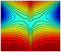
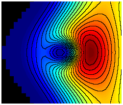
Chart
Auto2Fit can be also used for plotting function chart
and data chart, especially for implicit function chart.
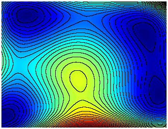
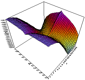
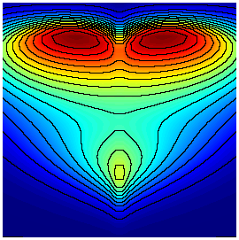
3D Chart Demo 1
|
Function
|

|
|
Code in Auto2Fit
|
Parameters
x[-1,1], y[-1,1], z;
PlotFunc
cos(z)/exp((sqrt(abs(x))-y)^2-x^2+y^2-z)-z=4;
|
|

|

|
Return
to top
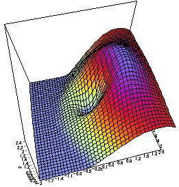
3D Chart Demo 2
|
Function
|

|
|
Code
in Auto2Fit
|
Parameters
x[-2,2],y[-2,2],z;
StepX
= 30;
StepY
= 30;
PlotFunction
z=(z^2+y^2+x^2-x*z)^0.25*(sin(5*(y^2+x^2)^0.1)^2+1-z^0.1+sin(x));
|
|

|

|
Return
to top
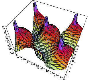
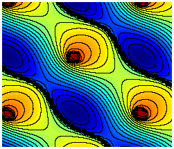
3D Chart Demo 3
|
Function
|

|
|
Code in Auto2Fit
|
Parameters
x[-6,2],y[-6,2],z;
StepX
= 50;
StepY
= 50;
PlotFunc
z=sin(z-x)*cos(z-y)-cos(x+y);
|
|

|

|
Return
to top
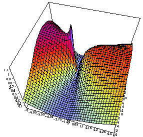
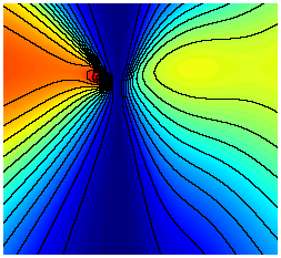
3D Chart Demo 4
|
Function
|

|
|
Code in Auto2Fit
|
Const
a=2, b=2.2, c=3.1, d=1.2;
Parameters
x[-8,6], y[-12,5],z;
StepX
= 40;
StepY
= 40;
PlotFunc
z= sqrt((x+a+z^(x^2/8))^2 + cos(z)*sin(z)^2*(y+b)^2)
- sqrt(z*(x+c)^2 + z*(y+d-z)^2);
|
|

|

|
Return
to top
3D Chart Demo 5
|
Function
|

|
|
Code in Auto2Fit
|
Parameters
x[0.5,5], y[0.5,5], z;
StepX
= 40;
StepY
= 40;
Plotfunction
4*cos(x*y+sin(x^z)^2)+sinh(x-y+z)+x/y+2.5-2*x^sin(x)+y^2/x+sin(z);
|
|

|

|
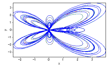
2D
Chart Demo 1
|
Function
|


|
|
Code
in Auto2Fit
ConstStr
t = i*(u+20*i);
Parameters
u[0,3*pi],x,y;
StepX
= 1200;
PlotParaFunction
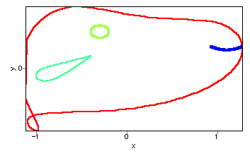
Plot(i=1:5)(x=cos(t)*(exp(cos(t))-2*cos(4*t)-sin(t/12)^5),
y=sin(t)*(exp(cos(t))-2*cos(4*t)-sin(t/12)^5));
|

|
Return
to top
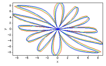
2D
Chart Demo 2
|
|
|
|
Code
in Auto2Fit
Constant
a=3,n=6;
ConstStr
r = a^2*cos(n*t+i*0.1);
Parameters
t[-pi,pi],x,y;
StepX
= 440;
PlotParaFunction
Plot(i=1:5)(x=r*cos(t+x^2*0.01),y=r*sin(t));
|

|
Return
to top
2D
Chart Demo 3
|
Function
|


|
|
Code
in Auto2Fit
Title
"Type your title here";
Parameters
t[0,2*pi], x, y;
Constant
a=2;
StepX
= 440;
PlotParaFunction
x=a*cos(t-0.4/a-0.1*x)^2, y=a*sin(t+0.03-x^2)^3
;
|

|
Return
to top
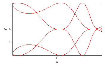
2D
Chart Demo 4
|
|
|
|
Code
in Auto2Fit
Title
"Snop";
Parameters
t[0,2*pi],x,y;
StepX
= 150;
PlotParaFunc
x=sin(t+x^2+y^2)+sin(t), y=cos(t+y);
x=0.1*sin(t)-0.3,
y=0.1*cos(t)+0.6;
x=0.3*sin(t-x^2)-0.7,
y=0.2*sin(t);
x=cos(t)/6+1.1,
y=cos(t)^2/20+0.3;
|

|
Return
to top
2D
Chart Demo 5
|
|
|
|
Code
in Auto2Fit
Parameters
t[0,2*pi],x,y;
StepX
= 210;
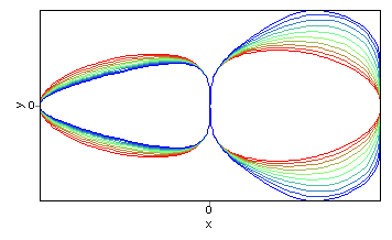
PlotParaFunction
Plot(i=1:10)(x=sin(t)^3, y=cos(t-y*x*i*0.1)*sin(t+y*x*0.1*i));
|

|
Return
to top
6. Miscellaneous
6.1.
Magic Matrix
This
is very interesting optimization problem on order:
A
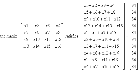
4 by 4 matrix consist of numbers for 1 to 16, the sum of every
row, column and corner-corner should be equal to 34 all. How
to construct such matrix?

| Codes
in Auto2Fit
|
Results
form Auto2Fit
|
| Title
"Magic Matrix";
Constant
S = 34;
Parameters
x(1:16)[1,16,0];
Exclusive
= true;
Function
x1 + x2 + x3 + x4 =
S;
x5
+ x6 + x7 + x8 =
S;
x9
+ x10 + x11 + x12 = S;
x13
+ x14 + x15 + x16 = S;
x1
+ x5 + x9 + x13 =
S;
x2
+ x6 + x10 + x14 = S;
x3
+ x7 + x11 + x15 = S;
x4
+ x8 + x12 + x16 = S;
x1
+ x6 + x11 + x16 = S;
x4
+ x7 + x10 + x13 = S;
|
"Magic
Matrix"
======
Results ======
Iterations:
2028
Elapsed
Time (Hr:Min:Sec:Msec): 00:00:02:690
Stop
Reason: RMSE reached
Algorithms:
Genetic Algorithms
x1:
2
x2:
9
x3:
8
x4:
15
x5:
16
x6:
7
x7:
10
x8:
1
x9:
13
x10:
6
x11:
11
x12:
4
x13:
3
x14:
12
x15:
5
x16:
14
Min.
Error: 0
|
Return
to top
6.2.
Calculator
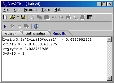
Auto2Fit
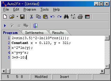
can also be used simply as a calculator by inputing plane text
|
Inputs
|
Outputs
|
|

|

|
Return
to top
6.3.
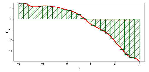
Integration
The
function is defined as below. Note it is an implicit function.

The
codes will draw function chart and calculate integration in
the range [-2, 3]
|
Codes in Auto2Fit
|
Outputs from Auto2Fit
|
|
Parameters
x[-2,3], y;
Integration
= 1;
PlotFunction
cos(y+x^2)^2+exp(x+y)*(1+sin(y)^3+x^2)-4=0;
|
"Draw
2-D Function Chart Demo 2"
Completion:
51/51
Failed
Points: 0
Elapsed
Time: 0:00:00
Algorithms:
Differential Evoluation(Scheme 1, Route 1)
Integral
Value of "cos(y+x^2)^2+exp(x+y)*(1+sin(y)^3+x^2)-4-(0)":
7.3028113
x y Residue
of "cos(y+x^2)^2+exp(x+y)*(1+sin(y)^3+x^2)-4-(0)" Integration
-2.000000 1.471077 0.000000
-1.900000 1.520360 0.000000 0.302739
-1.800000 1.529639 0.000000
-1.700000 1.472205 0.000000 0.594875
|

Return
to top
|

